 A. Khatib
Random Forest on Credit Card Approval Classification

This is an excerpt from my Kaggle notebook where I used a Random Forest classifier on credit card data (https://www.kaggle.com/datasets/rohitudageri/credit-card-details/data).
Random Forest was extremely easy to use and offer great insights into the data relatively quickly.
Exploring the Data
The CSV had a total 1548 rows, the table below shows the top 10 rows and with an additional column "Approved" that is 1 or 0
| CHILDREN | Annual_income | Birthday_count | Employed_days | Mobile_phone | Work_Phone | Phone | EMAIL_ID | Family_Members | Approved | |
|---|---|---|---|---|---|---|---|---|---|---|
| count | 1548.000000 | 1.525000e+03 | 1526.000000 | 1548.000000 | 1548.0 | 1548.000000 | 1548.000000 | 1548.000000 | 1548.000000 | 1548.000000 |
| mean | 0.412791 | 1.913993e+05 | -16040.342071 | 59364.689922 | 1.0 | 0.208010 | 0.309432 | 0.092377 | 2.161499 | 0.113049 |
| std | 0.776691 | 1.132530e+05 | 4229.503202 | 137808.062701 | 0.0 | 0.406015 | 0.462409 | 0.289651 | 0.947772 | 0.316755 |
| min | 0.000000 | 3.375000e+04 | -24946.000000 | -14887.000000 | 1.0 | 0.000000 | 0.000000 | 0.000000 | 1.000000 | 0.000000 |
| 25% | 0.000000 | 1.215000e+05 | -19553.000000 | -3174.500000 | 1.0 | 0.000000 | 0.000000 | 0.000000 | 2.000000 | 0.000000 |
| 50% | 0.000000 | 1.665000e+05 | -15661.500000 | -1565.000000 | 1.0 | 0.000000 | 0.000000 | 0.000000 | 2.000000 | 0.000000 |
| 75% | 1.000000 | 2.250000e+05 | -12417.000000 | -431.750000 | 1.0 | 0.000000 | 1.000000 | 0.000000 | 3.000000 | 0.000000 |
| max | 14.000000 | 1.575000e+06 | -7705.000000 | 365243.000000 | 1.0 | 1.000000 | 1.000000 | 1.000000 | 15.000000 | 1.000000 |
Modes
The table below shows the modes for all columns
| Field | Value |
|---|---|
| GENDER | F |
| Car_Owner | N |
| Propert_Owner | Y |
| CHILDREN | 0.0 |
| Annual_income | 135000.0 |
| Type_Income | Working |
| EDUCATION | Secondary / secondary special |
| Marital_status | Married |
| Housing_type | House / apartment |
| Employed_days | 365243.0 |
| Mobile_phone | 1.0 |
| Work_Phone | 0.0 |
| Phone | 0.0 |
| Type_Occupation | Laborers |
| Family_Members | 2.0 |
| Approved | 0.0 |
| Status | Declined |
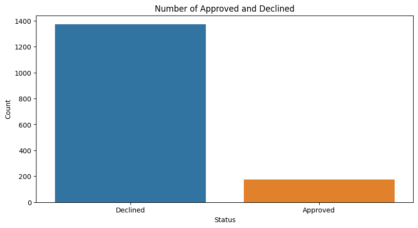
Number of Approved vs Declined
Note the data is heavily skewed to "Declined", this will be important later when fitting the model.
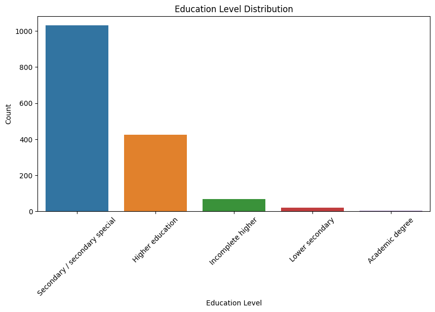
Education Distribution
Mostly high school and junior college.
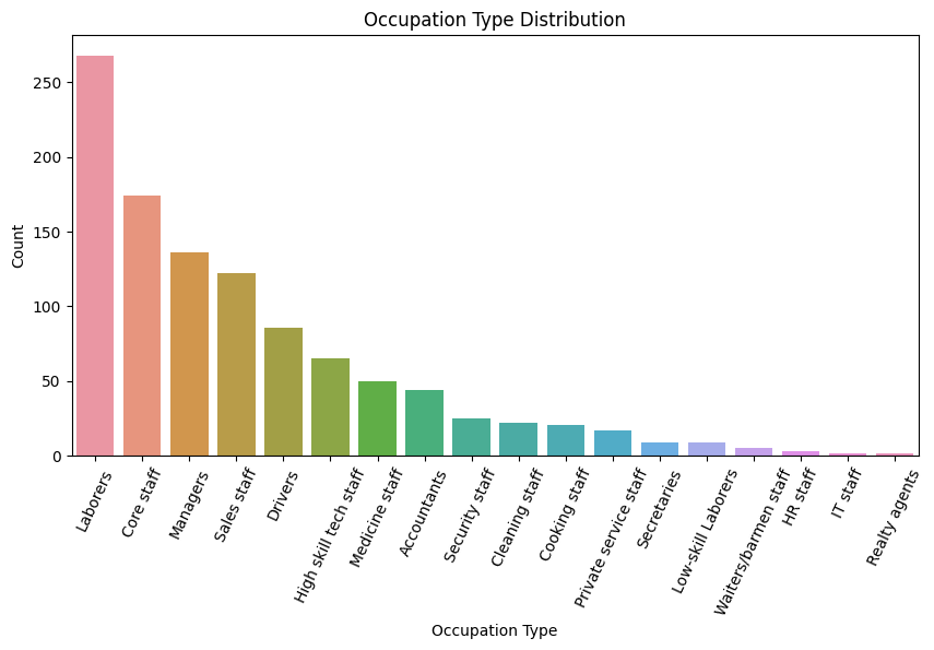
Occupation Type Distribution
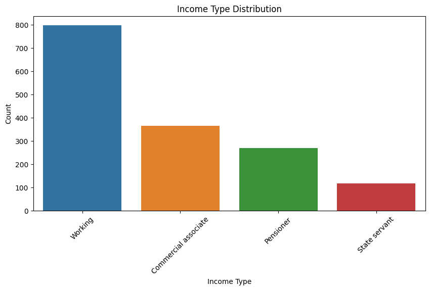
Income Type Distribution
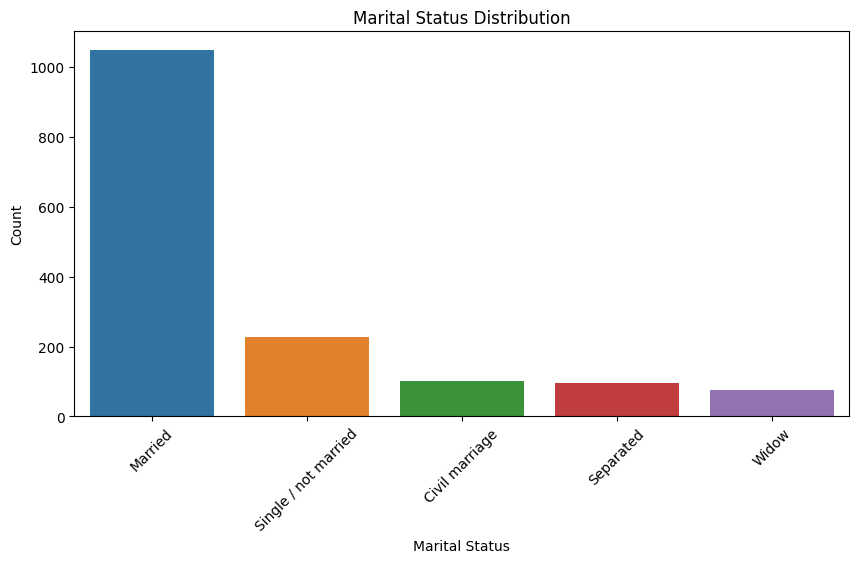
Marital Status Distribution
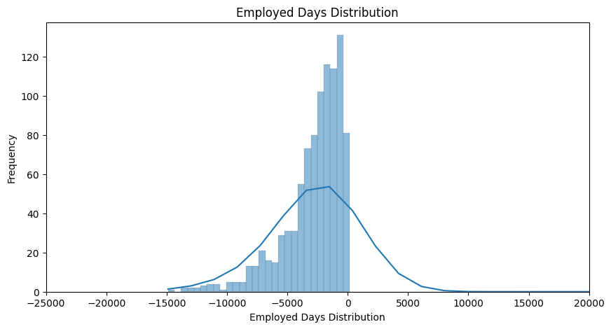
Employed Days Distribution
This looks odd, but, it's the start day of the job backwards from the current day (0). A positive number means the person is currently unemployed (currently at the time of collection). Mostly around 5-7 years employment
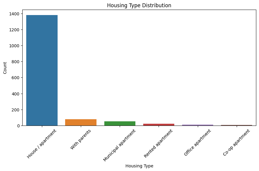
Housing Type Distribution
Preprocess Data
We'll first separate the categorical and continuous fields.
| Categorical | Continous |
|---|---|
| GENDER | CHILDREN |
| Car_Owner | Family_Members |
| Propert_Owner | Annual_income |
| Type_Income | Age |
| EDUCATION | EmployedDaysOnly |
| Marital_status | UnemployedDaysOnly |
| Housing_type | |
| Mobile_phone | |
| Work_Phone | |
| Phone | |
| Type_Occupation | |
| EMAIL_ID |
- Age is calculated in years from the
birthday_countfield. - Two new fields are added that count the number of employed days and unemployed days for each person
Random Forest Classifier
- Given how skewed the classes are, over sampling is needed.
- Given how small the dataset is, undersampling won't be used.
X, y = df[cats + conts].copy(), df[dep]

X_over, y_over = RandomOverSampler().fit_resample(X, y)

X_train, X_val, y_train, y_val = train_test_split(X_over, y_over, test_size=0.25)

X_train[cats] = X_train[cats].apply(lambda x: x.cat.codes)
X_val[cats] = X_val[cats].apply(lambda x: x.cat.codes)
rf = RandomForestClassifier(100, oob_score=True)
rf.fit(X_train, y_train);
| Metric | Value |
|---|---|
| MSE | 0.011644832605531296 |
| OOB | 0.013598834385624037 |
| Accuracy | 0.9883551673944687 |
| F1 Score | 0.988235294117647 |
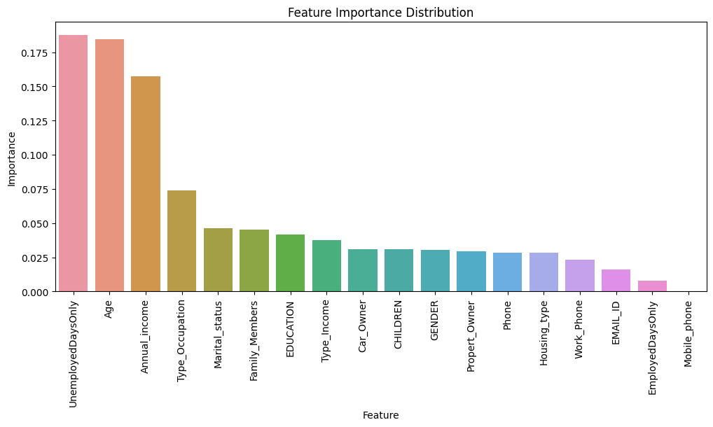
Feature Importance
And now my favorite part! This plot shows the most influential fields in the data. These are the ones that have the highest split ratio. No surprise length of employment and age are the 2 dominant factors. Annual income a close 3rd. So much data analysis can be condensed into the feature importance plot!
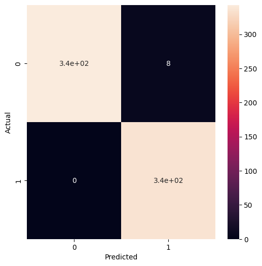
Confusion
There were no cases where the model predicted a "Declined" result where the actual status was "Approved". So the model is very good and accurately declining a credit approval. But it's a little too lenient where it predicted 8 would get approved when they were actually declined.
confusion = confusion_matrix(y_val, preds)
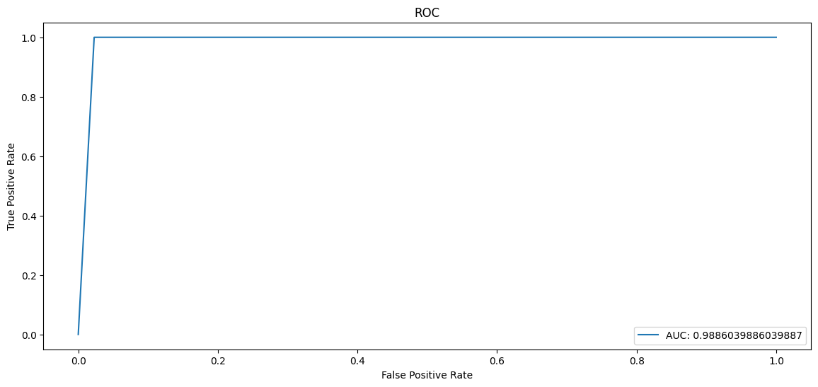
It follows that the ROC curve would almost be perfect, with AUC 0.988
Results
This was a non-starter without oversampling. Without oversampling, accuracy was deceptively pretty good around 91% but when looking at the confusion matrix and abismal F1 score it was obviously aweful.
I split employed days column into "unemployed" and "employed". It's not surprising looking at the feature importance plot that unemployed days, age and income are the top contributors.
Final Results:
| Score | Value |
|---|---|
| ROC AUC | 0.9958 |
| MSE | 0.0044 |
| OOB | 0.0141 |
| Accuracy | 0.9956 |
| F1 Score | 0.9955 |