
Testing Full State Feedback Controller on Nonlinear Pendulum Dynamics
We'll observe the response of a simple nonlinear pendulum by using a control law derived from linear analysis and test its performance.
We'll observe the response of a simple nonlinear pendulum by using a control law derived from linear analysis and test its performance. The linear model was easily stabilized as expected and is valid for initial conditions that are close to the equilibrium point. But what happens when we test the same controller on the nonlinear system? We should expect to see some different results.
Starting with the control law from the previous post on [full state feedback control for a simple pendulum](/articles/simple-state-space-model-of-a-pendulum), we want to test the controller's performance and observe the response of the nonlinear system.
\begin{equation} \begin{alignedat}{1} \dot{x}_{1} &= x_{2} \\ \dot{x}_{2} &= -p \sin{x_{1}} + u \end{alignedat} \end{equation}With full state feedback control given by $u = -Kx$, I used MATLAB's *place* command so that the poles of $(A-BK)$ are at desired locations.
K = place(A, B, poles);
% ex: poles = [-1 -2], K = [2.25 2]
To simulate the nonlinear dynamics, **Simulink** makes visualizing the system relatively easy. I start building the model by defining the expressions on the right-hand side of the dynamics equations using the *Fcn* blocks. Then simply add the $\frac{1}{s}$ *Integrator* block as shown.
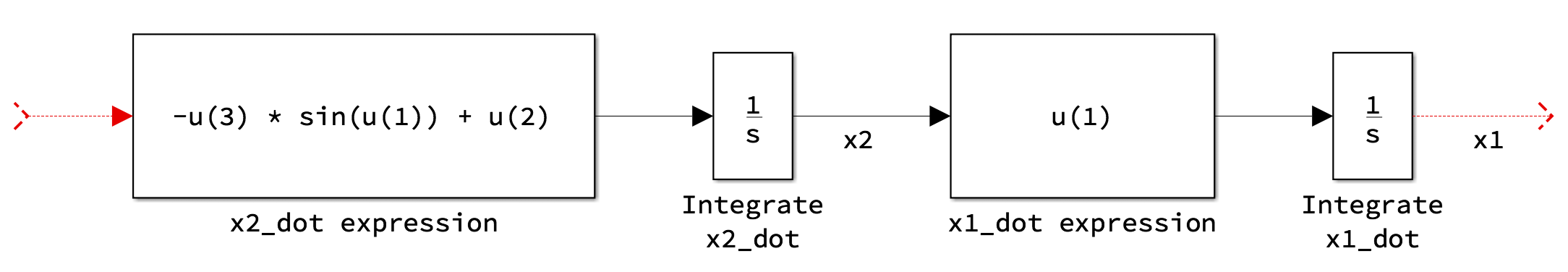
Notice that the first block on the left has a few *u(.)'s* indexed *1,2,3*, the input to this block is an array and can be created with a *mux* as shown. The indices in the expression corresponding to the order of the inputs of the Mux bar. We'll also add a mux at the right that represents our final state $x$.
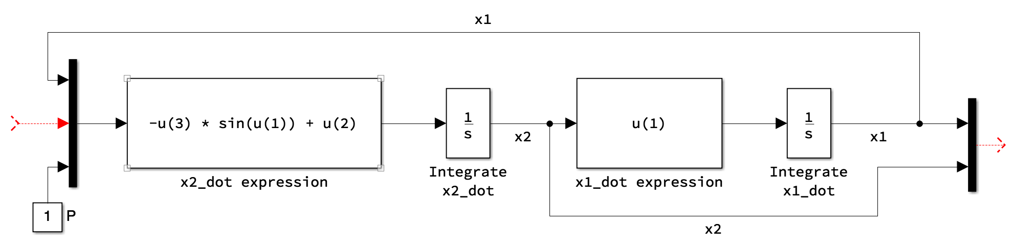
The above model now depicts the open-loop dynamics of the pendulum, there is no feedback control yet, hence open-loop, and the parameter $p$ is currently a constant, lumping the terms $\frac{g}{l}$.
In the [previous post](/articles/6) the system was transformed so that the equilibrium point is the origin of the state-space. We can do the same here and stabilize to the origin by defining a new term:
\begin{equation} \begin{alignedat}{0} g = x - x^* \\ \text{where $x^*$ is an equilibrium point} \end{alignedat} \end{equation}Substituting for $x = y + x^*$, transforms the equations into the form [[1]](#cite):
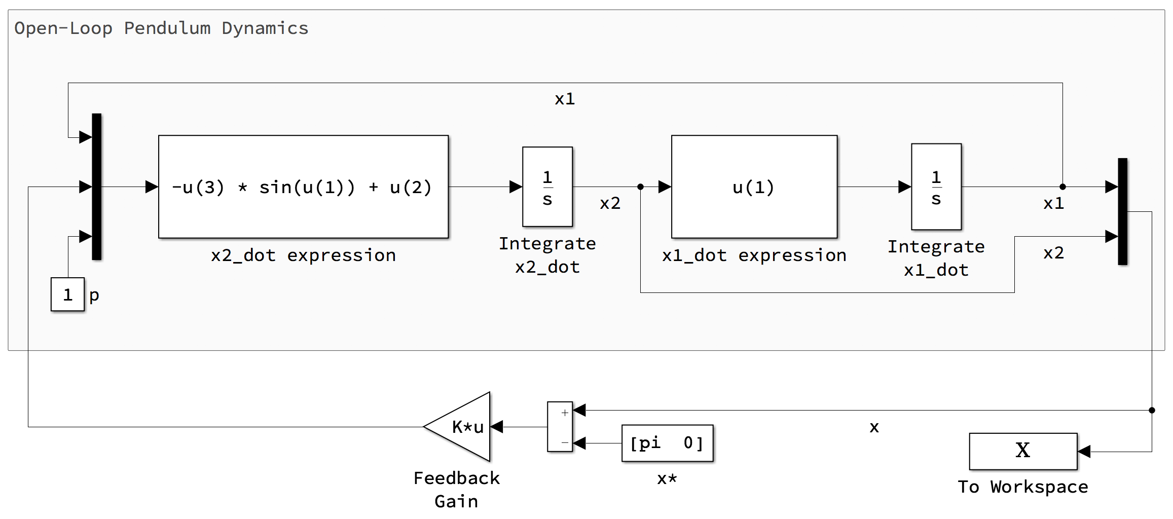
\begin{gather*} \dot{y} = f(y + x^*) \end{gather*}But for clarity I'll leave the block diagram unchanged and simply calculate the error term $e = x - x^*$ prior to calculating the gain, so that the feedback control gain becomes:
\begin{gather*} -K(x - x^*) \\ \text{where $x^* = [\pi; 0]$} \end{gather*}% Full state feedback control law on nonlinear pendulum model.
clear; clc;
k = 1;
legendInfo = {};
figure(1);
% Increase the initial angle offset from the inverted position
% This ranges from small to large offsets, remember that the system
for m = pi*0.95:-pi/4:0
set_param('Pendulum/Integrate x1_dot', 'InitialCondition', num2str(m));
% Run the Simulink model
sim('Pendulum');
x1 = X.Data(:,1);
plot(tout, x1, 'LineWidth', 2);
xlabel('Time $s$', 'Interpreter', 'LaTex', 'FontSize', 16);
ylabel('Angle $x_1$', 'Interpreter', 'LaTex', 'FontSize', 16);
legendInfo{k} = ['$x_{1_{IC}}$ = ' num2str(m)];
hold on;
k = k + 1;
end
hold off;
legend(legendInfo, 'Interpreter', 'LaTex', 'FontSize', 16);
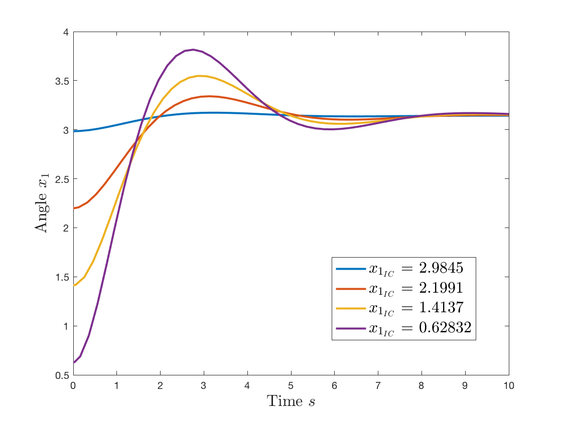
The MATLAB code above runs the Simulink model with different initial angle offsets eg: *near* the equilibrium point $\pi$ and large offset at the downward verticle $x_1=0$. The *To Workspace* block saves the response for $x$ so we can plot and inspect the time-series data.
The plots above show the performance difference of the nonlinear system using the control law from the linear analysis. The performance of the linear system is better as expected since we are not taking into account the nonlinearities that arise when perturbations are far from the nominal trajectories.
As is expected, the nonlinear response is very similar to the linear system when initial conditions are small. But notice that as the angle offset increase, the nonlinear term begins to affect the response.
The Simulink model and MATLAB code for the Testing Nonlinear Pendulum is available for download so you can try different control gains and parameters.
References
- Jean-Jacques E. Slotine and Weiping Li, "Applied Nonlinear Control," Prentice Hall, Englewood Cliffs, New Jersey 07632, 1991