Hill Model Simulation and Functional Electrical Stimulation
While some have characterized the wrist as a second order system, the focus here is fitting a more complex fourth order model that accurately represents observed responses and muscle activity [1].
While some have characterized the wrist as a second order system, the focus here is fitting a more complex fourth order model that accurately represents observed responses and muscle activity [1].
Prior to the publishing of [1], most studies of the wrist did not include an explicit model when analyzing responses.
Using this model and Hill’s equation relating force and velocity with electromyograms (EMG), a controller can be designed that correctly activates the wrist muscles to achieve desired movements. Furthermore, characterizing the wrist using this model lends itself to a straightforward approach to designing a functional electrical stimulation (FES) system.
Terms and Definitions
Alpha motor neurons are responsible for direct activation of skeletal muscles. Motor units include the alpha motor neuron and all of the muscle fibers which it is responsible for activating. Muscle fiber is the strand of tissue that includes the myofibrils at its core, activated by the axon attached at its surface. Muscle fibril or myofibril makes up the core of the muscle fiber. Myofilaments make up the myofibril and are constructed of proteins. The thin filament is activated by the thick filament, myosin. Actin is a protein that makes up the thin filament. Myosin attaches and pulls on the actin producing contraction. Sarcomere surrounds each filament and anchors the myosin fibers.
Fused tetanus is a contraction that does not have oscillations. Unfused tetanus is a contraction with unsteady contractions resulting in oscillations. Recruitment refers to the order in which muscles are activated, using muscles that fatigue slower first and resorting to faster fatiguing muscles last. Size principle refers to the excitability of small motor units opposed to larger ones. As signal strength increases, large motor units are recruited, gradually increasing contractile force.
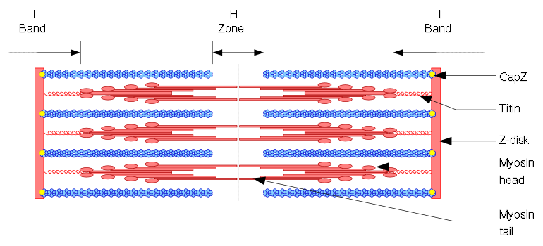
Figure 1 is the diagram for the muscle components. Observe that during contraction, the actin filaments move closer together reducing the H-Zone, and overlap during extreme conditions. This overlapping reduces the number of actin attachment sites to myosin. With less active area contract- ing, the force decreases.
The opposite condition during extreme extension causes the H-Zone to grow large enough that actin-myosin attachment sites decrease and in turn decrease force. This case reduces force more drastically than an extreme contraction where actin-myosin sites can still reattach during reduced contraction.
Linear Model Simulation
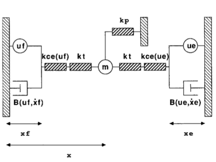
The objective is to measure isometric force produced by the wrist in response to a step input. Two values of stiffness are used during an equal and opposite contraction of the flexor and extensor muscles. The linear model is shown in figure 2 where $U_{e}$ and $U_{f}$ are the inputs. Stiffening of the muscles is a common problem after spinal cord injuries and this simulation will compare the response due to increased muscle stiffness.
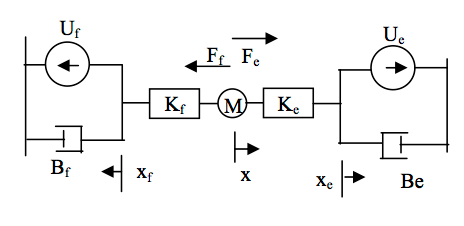
The equations of motion for the mass $m$ are as follows:
\begin{equation} \begin{alignedat}{1} m\ddot{x} &= F_{e} - F_{f} \ \end{alignedat} \end{equation}Where the forces are:
\begin{equation} \begin{alignedat}{1} F_{f} &= k_{f}(x + x_{f}) = U_{f} - B_{f}\dot{x}_{f} \\ F{e} &= -k_{e}(x + x_{e}) = U_{e} - B_{e}\dot{x}_{e} \\ F{p} &= -k_{p}x \end{alignedat} \end{equation}Since the damping terms are constant, we can define new variables and represent the dynamics as a set of first order equations. Let $x_{1} = x$, $x_{2} = \dot{x}$ and rearrange the above equations:
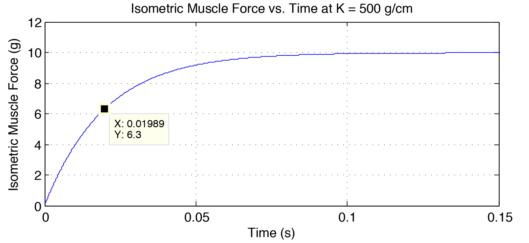
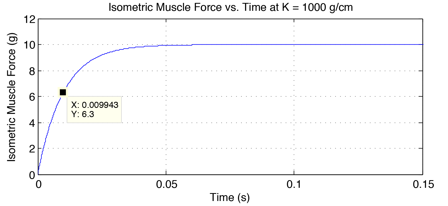
\begin{equation} \begin{alignedat}{1} \dot{x}_{1} &= x_{2} \\ \dot{x}_{2} &= \frac{1}{m}\left(-k_{f}\left(x_{1}+x_{f}\right) -k_{e}\left(x_{1} - x_{e}\right)\right) \\ \displaystyle\dot{x}_{f} &= \frac{1}{B_{f}} \left(U_{f} - k_{f}\left(x_{1} + x_{f}\right)\right) \\ \displaystyle\dot{x}_{e} &= \frac{1}{B_{e}} \left(U_{e} - k_{e}\left(x_{1} - x_{e}\right)\right) \\ \end{alignedat} \end{equation}Simulation of the dynamics is straight forward, requiring only the state space representation of the model and the step input. The response time is measured when the isometric muscle force reaches 6.3 grams. Figure 3 shows force vs time at a stiffness of 500 g/cm. The time required to generate this force is listed on the datatap as 0.01989 sec. When the stiffness is doubled in figure 4, the response time decreases, as expected, to 0.009943 sec.
The linear model with constant stiffness and damping is valid in a region around the equilibrium, but cannot be reliably extended to extreme cases or global stability. Nonlinear analysis in the next section will assume velocity and state dependent stiffness and damping.
Nonlinear Model Simulation
The objective is to move the wrist from an initial position at $10^\circ$ extension to a $20^\circ$ flexion as fast as possible. Equations of motion are formulated from the model shown in figure 4, and will be used to simulate responses with different parameters.
Writing $F=ma$ for the mass $m$:
\begin{equation} \begin{alignedat}{1} m\ddot{x} &= F_{e} - F_{f} - F_{p} \\ \end{alignedat} \end{equation}Where the forces are:
\begin{equation} \begin{alignedat}{1} F_{f} &= k_{f}(x + x_{f}) = U_{f} - B_{f}\dot{x}_{f} \\ F_{e} &= -k_{e}(x + x_{e}) = U_{e} - B_{e}\dot{x}_{e} \\ F_{p} &= -k_{p}x \end{alignedat} \end{equation}The viscosities $B_{f}$ and $B_{e}$ are not constant, they vary with velocity $\dot{x_{f}}$, $\dot{x_{e}}$ and active state $U_{f}$, $U{e}$. Using Hill's equation, the viscosities can be defined as follows and substituted back into the force equations.
\begin{equation} \begin{alignedat}{1} B_{f} = \frac{U_{f} + a}{\dot{x}_{f} + b}\\ B_{e} = \frac{U_{f} - a}{\dot{x}_{e} - b}\\ \end{alignedat} \end{equation}Now we can define new variables and represent the dynamics as a set of first order equations. Let $x_{1} = x$, $x_{2} = \dot{x}$ and rearrange the above equations:
\begin{equation} \begin{alignedat}{1} \dot{x}_{1} &= x_{2} \\ \dot{x}_{2} &= \frac{1}{m}\left(-k_{f}\left(x_{1}+x_{f}\right) -k_{e}\left(x_{1} - x_{e}\right) - k_{p}x_{1}\right) \\ \displaystyle\dot{x}_{f} &= \frac{\left(U_{f} - k_{f}\left(x_{1} + x_{f}\right) \right)b}{ a + k_{f}\left(x_{1} + x_{f}\right)} \\ \displaystyle\dot{x}_{e} &= \frac{\left(U_{e} - k_{e}\left(x_{1} - x_{f}\right) \right)b}{ a - k_{f}\left(x_{1} - x_{e}\right)} \\ \end{alignedat} \end{equation}Where the stiffnesses are also dependent on active state and defined:
\begin{equation} \begin{alignedat}{1} \displaystyle k_{f} = \frac{k_{t}k_{ce}U_{f}}{k_{t} + k_{ce}U_{f}} \\ \displaystyle k_{e} = \frac{k_{t}k_{ce}U_{e}}{k_{t} + k_{ce}U_{e}} \end{alignedat} \end{equation}With the equations now in first order form, MATLAB can be used to integrate the dynamics and a control law designed with $U_{f}$ and $U_{e}$ as inputs and $x_{1}$ as output wrist angle. The variables $a$ and $b$ and control input are free parameters and can be chosen by trial and error or by optimizing a cost function.
Simulation and Optimization
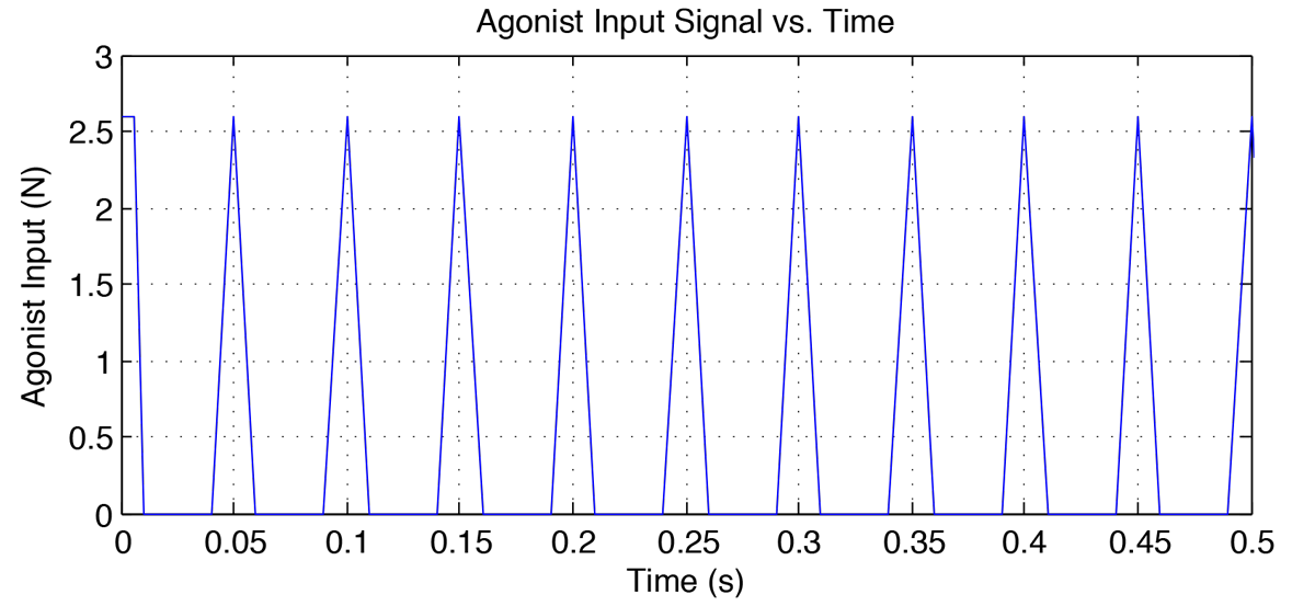
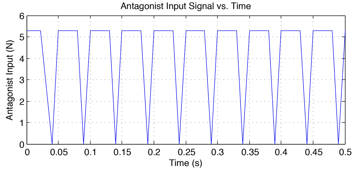
The dynamics are simulated using Simulink where the equations are integrated simultaneously with a variety of input signals. Trial and error approach is used to determine $a$ and $b$ knowing from equation 4 that increasing $a$ and decreasing $b$ will increase the viscous damping terms. Parameters of the input functions are also determined by systematically adjustment of amplitude, frequency, pulse width and the degree of interleaving.
The simulation and recorded results of the agonist and antagonist muscle reveal that a fast response depends on activity of both muscles at delayed intervals. Using this strategy to design the control inputs, square wave pulses are interleaved to increase overall stiffness and drive the wrist to the target. Fast responses resulted in oscillations, however by varying $a$ and $b$ to adjust the damping, a reasonable response is obtained.
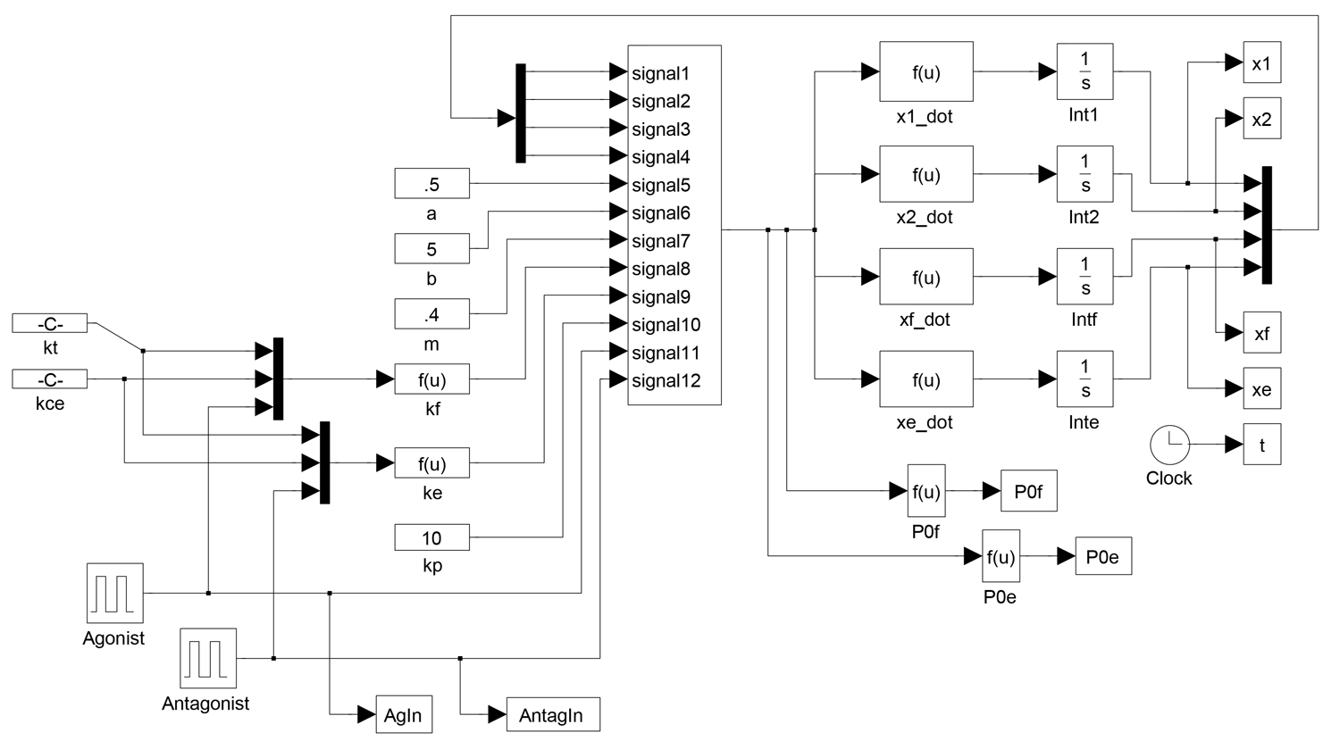
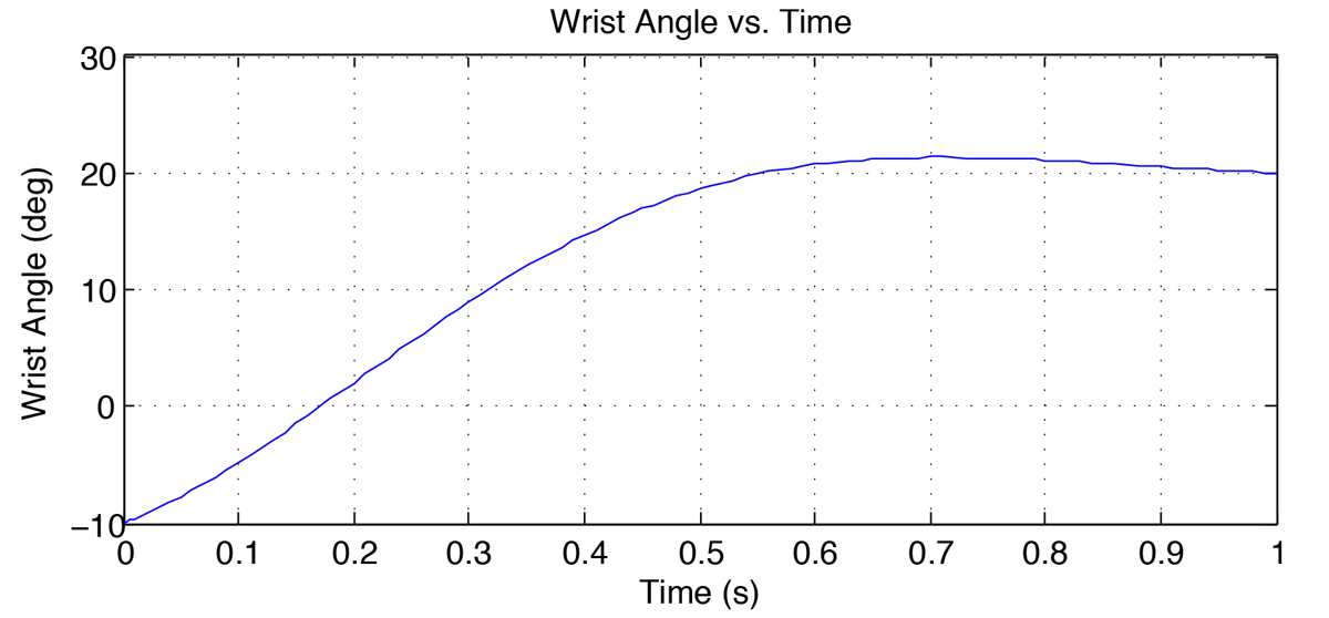
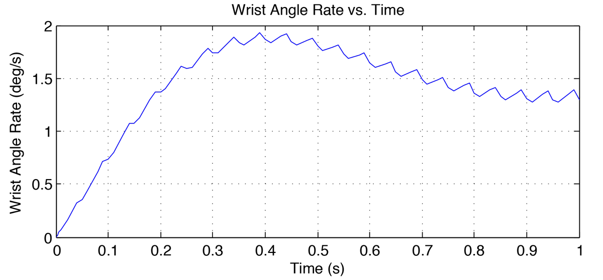
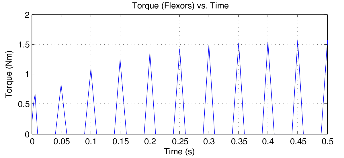
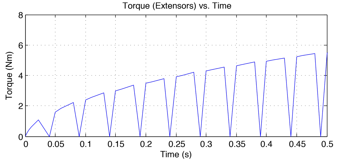
The simulink model is shown in figure 6 below. Figures 7-8 show the wrist trajectory as it moves to the target and the velocity during the movement. Figures 9-10 show the agonist and antagonist muscle input signals. Figures 11-12 show the torques in the flexor and extensor muscles over the time period. Observe that the maximum torques in either muscle do not exceed the muscles' maximum torques.
Conclusions
Observe from figure 7, the time required to move from $1^\circ$ away from initial to within $1^\circ$ of the final target is $0.46 sec$. This is significantly slower compared to the results from [1] where the same response is executed in around $0.25 sec$. However, this simulation does not include a parameter optimization algorithm.
Using an explicit model to describe the wrist response allows for systematic design of an FES system. Activating the agonist and antagonist muscles of the model produce a response very close to that of the actual hand [1]. Since muscle stimulations are explicitly known, they can be reconstructed and optimized for each patient.
As stated, the muscles of the wrist are accessible for EMG measurement and likewise for surface stimulation. Varieties of movements can be obtained by adjusting the stimulation parameters and/or the interleaving of signals. Though torques were below maximum levels, stimulation strength may exceed thresholds. However, with a functional model, many nonlinear control strategies can be tested for advantages and customized for each patient.
MATLAB Code & Model
Below is the code to run the linear model.
% Linear Model Simulation of the Wrist
clear; close all; clc;

% Define the variables of the system as real numbers (symbolic)
syms x1 x2 xf xe x Uf Ue real

K = 500; % Stiffness
B = 10; % Damping
m = 500; % Mass

kf = K; ke = K;
Bf = B; Be = B;

t = 0:.0001:.4;

% State-Space Equations of Motion
Am(1,:) = [0 1 0 0];
Am(2,:) = [(1/m)*(-ke - kf) 0 -kf/m ke/m];
Am(3,:) = [-kf/Bf 0 -kf/Bf 0];
Am(4,:) = [ke/Be 0 0 -ke/Be];

U = [Uf Ue]';

Bm = [0 0; 0 0; 1/Bf 0; 0 1/Bf];

Cm = [1 0 1 0];
Dm = 0;

Sys = ss(Am, Bm, Cm, Dm);

[y,t,x] = step(10*Sys, t);

h = figure(1);
set(h, 'position',[500 500 600 250])
plot(t, y(:,1)*K); grid on;
title('Isometric Muscle Force vs. Time at K = 500 g/cm');
xlabel('Time (s)'); ylabel('Isometric Muscle Force (g)');
axis([0 0.15 0 12])
Download the MATLAB code and Simulink Model to try out the nonlinear Hill Model simulation.
References
- S.L. Lehman and B.M. Calhoun, ``An Identified Model for Human Wrist Movements," Experimental BrainResearch, 1989